Frutas entre fechas

Tenemos una columna con frutas, cada fruta tiene asignada una serie de fechas.

Debemos de encontrar la lista de productos (ordenados alfabéticamente) para el rango de fechas que figura en las columnas H e I de la tabla que figura en las columnas A a F.

Lo vamos a realizar de dos formas.

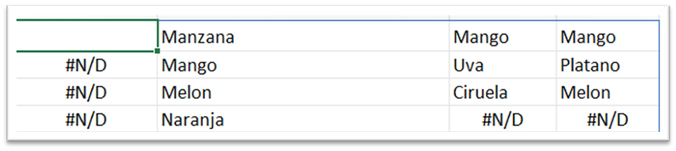
En la celda H6, usamos LET, creamos una variable, y, transponemos el rango A2:F8.

=LET(xx;TRANSPONER(A2:F8);xx)

Tenemos una matriz desbordada de siete columnas, con cada producto, y, de cada producto cuelgan las fechas asociadas a cada producto.

Creamos otra variable, usamos la funcion ELERGIRFILAS, como argumento matriz, ponemos la variable “xx”, como argumento número de fila1, ponemos 1, nos vamos a traer la primera fila que contiene las frutas.

=LET(xx;TRANSPONER(A2:F8);yy;ELEGIRFILAS(xx;1);yy)

Creamos otra variable, usamos la funcion SECUENCIA, omitimos el argumento filas, como argumento columnas, ponemos 3, como argumento inicio, seleccionamos la celda H2.

=LET(xx;TRANSPONER(A2:F8);yy;ELEGIRFILAS(xx;1);ww;SECUENCIA(;3;H2);ww)

Tenemos el rango de fechas por las que buscar.

Creamos otra variable, ponemos la variable “xx” e igualamos a la primera columna de la variable “ww”, para ello, usamos la funcion TOMAR, como argumento matriz, ponemos la variable “ww”, omitimos el argumento filas, como argumento columnas, ponemos 1.

=LET(xx;TRANSPONER(A2:F8);yy;ELEGIRFILAS(xx;1);ww;SECUENCIA(;3;H2);a;xx=TOMAR(ww;;1);a)

Tenemos una matriz desbordada con VERDADERO donde hay coincidencia con la primera fecha, y, FALSO donde no hay coincidencia.

Creamos otra variable, volvemos a poner la variable “xx” e igualamos a la segunda columna de la variable “ww”, para ello, usamos la funcion ELEGIRCOLS, como argumento matriz, ponemos la variable “ww”, como argumento numero de columna1, ponemos 2.

=LET(xx;TRANSPONER(A2:F8);yy;ELEGIRFILAS(xx;1);ww;SECUENCIA(;3;H2);a;xx=TOMAR(ww;;1);b;xx=ELEGIRCOLS(ww;2);b)

Obtenemos una matriz desbordada como para la variable “a” pero con coincidencia para la segunda fecha.

Creamos otra variable, igualamos la variable “xx” a la última columna de la variable “ww”, para ello, usamos la funcion TOMAR, como argumento matriz, ponemos la variable “ww”, omitimos el argumento filas, como argumento columnas, ponemos -1.

=LET(xx;TRANSPONER(A2:F8);yy;ELEGIRFILAS(xx;1);ww;SECUENCIA(;3;H2);a;xx=TOMAR(ww;;1);b;xx=ELEGIRCOLS(ww;2);c;xx=TOMAR(ww;;-1);c)

Obtenemos una matriz desbordada igual que para las variables “a” y “b”, pero, para la tercera fecha.

Creamos otra variable, usamos el condicional SI, preguntamos si la variable “a” es igual a VERDADERO, en ese caso, que devuelva la variable “yy”, en caso contrario, que devuelva error.

=LET(xx;TRANSPONER(A2:F8);yy;ELEGIRFILAS(xx;1);ww;SECUENCIA(;3;H2);a;xx=TOMAR(ww;;1);b;xx=ELEGIRCOLS(ww;2);c;xx=TOMAR(ww;;-1);d;SI(a;yy;NOD());d)

Tenemos una matriz desbordada con las frutas donde coincide con la primera fecha, y, error donde no hay coincidencia.

Usamos la funcion ENCOL, como argumento matriz, es el condicional SI, como argumento ignorar, seleccionamos 3.

=LET(xx;TRANSPONER(A2:F8);yy;ELEGIRFILAS(xx;1);ww;SECUENCIA(;3;H2);a;xx=TOMAR(ww;;1);b;xx=ELEGIRCOLS(ww;2);c;xx=TOMAR(ww;;-1);d;ENCOL(SI(a;yy;NOD());3);d)

Tenemos las frutas que corresponden con la primera fecha en vertical.

Ordenamos.

=LET(xx;TRANSPONER(A2:F8);yy;ELEGIRFILAS(xx;1);ww;SECUENCIA(;3;H2);a;xx=TOMAR(ww;;1);b;xx=ELEGIRCOLS(ww;2);c;xx=TOMAR(ww;;-1);d;ORDENAR(ENCOL(SI(a;yy;NOD());3));d)

Usamos la funcion UNIRCADENAS, como argumento delimitador, entre comillas dobles, ponemos coma y dejamos un espacio, ignoramos celdas vacías, u. omitimos el argumento, como argumento texto1, es la funcion ORDENAR.

=LET(xx;TRANSPONER(A2:F8);yy;ELEGIRFILAS(xx;1);ww;SECUENCIA(;3;H2);a;xx=TOMAR(ww;;1);b;xx=ELEGIRCOLS(ww;2);c;xx=TOMAR(ww;;-1);d;UNIRCADENAS(", ";VERDADERO;ORDENAR(ENCOL(SI(a;yy;NOD());3)));d)

Ya tenemos ordenadas las frutas para la primera fecha.

Creamos otra variable, repetimos la expresión para la variable “d”, pero, cambiamos el argumento prueba lógica del condicional SI por la variable “b”.

=LET(xx;TRANSPONER(A2:F8);yy;ELEGIRFILAS(xx;1);ww;SECUENCIA(;3;H2);a;xx=TOMAR(ww;;1);b;xx=ELEGIRCOLS(ww;2);c;xx=TOMAR(ww;;-1);d;UNIRCADENAS(", ";VERDADERO;ORDENAR(ENCOL(SI(a;yy;NOD());3)));e;UNIRCADENAS(", ";VERDADERO;ORDENAR(ENCOL(SI(b;yy;NOD());3)));e)

Tenemos ordenadas las frutas para la segunda fecha.

Repetimos la operación anterior, y, cambiamos la variable “b” por la variable “c”.

=LET(xx;TRANSPONER(A2:F8);yy;ELEGIRFILAS(xx;1);ww;SECUENCIA(;3;H2);a;xx=TOMAR(ww;;1);b;xx=ELEGIRCOLS(ww;2);c;xx=TOMAR(ww;;-1);d;UNIRCADENAS(", ";VERDADERO;ORDENAR(ENCOL(SI(a;yy;NOD());3)));e;UNIRCADENAS(", ";VERDADERO;ORDENAR(ENCOL(SI(b;yy;NOD());3)));f;UNIRCADENAS(", ";VERDADERO;ORDENAR(ENCOL(SI(c;yy;NOD());3)));f)

Tenemos ordenadas las frutas para la tercera fecha.

Usamos el argumento calculo de LET, usamos la funcion APILARV, como argumento matriz1, ponemos la variable “d”, como argumento matriz2, ponemos la variable “e”, como argumento matriz3, ponemos la variable “f”.

=LET(xx;TRANSPONER(A2:F8);yy;ELEGIRFILAS(xx;1);ww;SECUENCIA(;3;H2);a;xx=TOMAR(ww;;1);b;xx=ELEGIRCOLS(ww;2);c;xx=TOMAR(ww;;-1);d;UNIRCADENAS(", ";VERDADERO;ORDENAR(ENCOL(SI(a;yy;NOD());3)));e;UNIRCADENAS(", ";VERDADERO;ORDENAR(ENCOL(SI(b;yy;NOD());3)));f;UNIRCADENAS(", ";VERDADERO;ORDENAR(ENCOL(SI(c;yy;NOD());3)));APILARV(d;e;f))

Usamos APILARH antes de APILARV, como argumento matriz1, usamos ENCOL, como argumento ponemos la variable “ww”, como argumento matriz2, es la función APILARV.

=LET(xx;TRANSPONER(A2:F8);yy;ELEGIRFILAS(xx;1);ww;SECUENCIA(;3;H2);a;xx=TOMAR(ww;;1);b;xx=ELEGIRCOLS(ww;2);c;xx=TOMAR(ww;;-1);d;UNIRCADENAS(", ";VERDADERO;ORDENAR(ENCOL(SI(a;yy;NOD());3)));e;UNIRCADENAS(", ";VERDADERO;ORDENAR(ENCOL(SI(b;yy;NOD());3)));f;UNIRCADENAS(", ";VERDADERO;ORDENAR(ENCOL(SI(c;yy;NOD());3)));APILARH(ENCOL(ww);APILARV(d;e;f)))

Aceptamos, y, ya lo tenemos.

Haciéndolo de esta forma, solo podemos trabajar con tres fechas, si el rango de fechas fuese de mas de tres fechas, solo contemplaría las tres primeras fechas.

Ahora, lo vamos a realizar de forma que sea dinámica.

Usamos LET, creamos una variable, usamos la funcion SECUENCIA, omitimos el argumento filas, como argumento columnas, ponemos 3, como inicio, seleccionamos la celda H2.

=LET(xx;SECUENCIA(;3;H2);xx)

Tenemos el rango de fechas por el que buscar.

Creamos otra variable, usamos la funcion ENCOL, como argumento matriz, seleccionamos el rango A2:A8, concatenamos con un guion medio, concatenamos con el rango B2:F8.

=LET(xx;SECUENCIA(;3;H2);a;ENCOL(A2:A8&"-"&B2:F8);a)

Tenemos en vertical, cada fruta separada por un guion medio y la fecha correspondiente.

Creamos otra variable, usamos la funcion DIVIDIRTEXTO, como argumento texto, ponemos la variable “a”, como argumento delimitador de columna, entre comillas dobles, ponemos el guion medio.

=LET(xx;SECUENCIA(;3;H2);a;ENCOL(A2:A8&"-"&B2:F8);b;DIVIDIRTEXTO(a;"-");b)

Tenemos las frutas.

Creamos otra variable, usamos la funcion TEXTODESPUES, como argumento texto, ponemos la variable “a”, como argumento delimitador, entre comillas dobles, ponemos el guion medio.

=LET(xx;SECUENCIA(;3;H2);a;ENCOL(A2:A8&"-"&B2:F8);b;DIVIDIRTEXTO(a;"-");c;TEXTODESPUES(a;"-");c)

Tenemos las fechas para cada fruta.

Vemos que las fechas están alineadas a la izquierda, quiere decir, que esta en formato de texto, pues, multiplicamos por 1 la funcion TEXTODESPUES.

=LET(xx;SECUENCIA(;3;H2);a;ENCOL(A2:A8&"-"&B2:F8);b;DIVIDIRTEXTO(a;"-");c;TEXTODESPUES(a;"-")*1;c)

Ya tenemos las fechas en formato de número, vemos que han quedado alineadas a la derecha, y, tenemos error donde era blanco.

Usamos la funcion SI.ERROR, como argumento valor es la funcion TEXTODESPUES, como argumento valor si error, ponemos blanco.

=LET(xx;SECUENCIA(;3;H2);a;ENCOL(A2:A8&"-"&B2:F8);b;DIVIDIRTEXTO(a;"-");c;SI.ERROR(TEXTODESPUES(a;"-")*1;"");c)

Creamos otra variable, usamos la funcion REDUCE, como argumento valor inicial, ponemos blanco, como argumento array, ponemos la variable “xx”, como argumento funcion ponemos LAMBDA, y, declaramos dos variables.

=LET(xx;SECUENCIA(;3;H2);a;ENCOL(A2:A8&"-"&B2:F8);b;DIVIDIRTEXTO(a;"-");c;SI.ERROR(TEXTODESPUES(a;"-")*1;"");d;REDUCE("";xx;LAMBDA(x;y

Como argumento cálculo de LAMBDA, usamos la función APILARH, como argumento matriz1, ponemos la variable “x”, como argumento matriz2, filtramos la variable “b”, siempre que la variable “c” sea igual a la variable “y”.

=LET(xx;SECUENCIA(;3;H2);a;ENCOL(A2:A8&"-"&B2:F8);b;DIVIDIRTEXTO(a;"-");c;SI.ERROR(TEXTODESPUES(a;"-")*1;"");d;REDUCE("";xx;LAMBDA(x;y;APILARH(x;FILTRAR(b;c=y))));d)

Ya tenemos las frutas que corresponden con cada fecha.

Ordenamos.

=LET(xx;SECUENCIA(;3;H2);a;ENCOL(A2:A8&"-"&B2:F8);b;DIVIDIRTEXTO(a;"-");c;SI.ERROR(TEXTODESPUES(a;"-")*1;"");d;REDUCE("";xx;LAMBDA(x;y;APILARH(x;ORDENAR(FILTRAR(b;c=y)))));d)

La primera columna está de más, usamos la funcion EXCLUIR, como argumento matriz es la funcion REDUCE, omitimos el argumento filas, como argumento columnas, ponemos 1.

=LET(xx;SECUENCIA(;3;H2);a;ENCOL(A2:A8&"-"&B2:F8);b;DIVIDIRTEXTO(a;"-");c;SI.ERROR(TEXTODESPUES(a;"-")*1;"");d;EXCLUIR(REDUCE("";xx;LAMBDA(x;y;APILARH(x;ORDENAR(FILTRAR(b;c=y)))));;1);d)

En cada columna, tenemos las frutas que pertenecen con cada fecha, pero, debemos de tenerlas en filas, creamos otra variable, y, transponemos la variable “d”.

=LET(xx;SECUENCIA(;3;H2);a;ENCOL(A2:A8&"-"&B2:F8);b;DIVIDIRTEXTO(a;"-");c;SI.ERROR(TEXTODESPUES(a;"-")*1;"");d;EXCLUIR(REDUCE("";xx;LAMBDA(x;y;APILARH(x;ORDENAR(FILTRAR(b;c=y)))));;1);e;TRANSPONER(d);e)

Usamos la función SI.ERROR, y, ponemos blanco donde es error.

=LET(xx;SECUENCIA(;3;H2);a;ENCOL(A2:A8&"-"&B2:F8);b;DIVIDIRTEXTO(a;"-");c;SI.ERROR(TEXTODESPUES(a;"-")*1;"");d;EXCLUIR(REDUCE("";xx;LAMBDA(x;y;APILARH(x;ORDENAR(FILTRAR(b;c=y)))));;1);e;SI.ERROR(TRANSPONER(d);"");e)

Usamos el argumento cálculo de LET, usamos la funcion BYROW, como argumento array, ponemos la variable “e”, como argumento funcion ponemos LAMBDA, declaramos una variable, como argumento cálculo de LAMBDA, usamos la funcion UNIRCADENAS, como argumento delimitador, entre comillas dobles, ponemos coma y dejamos un espacio, ignoramos celdas vacías, u, omitimos el argumento, como argumento texto1, ponemos la variable “x”.

=LET(xx;SECUENCIA(;3;H2);a;ENCOL(A2:A8&"-"&B2:F8);b;DIVIDIRTEXTO(a;"-");c;SI.ERROR(TEXTODESPUES(a;"-")*1;"");d;EXCLUIR(REDUCE("";xx;LAMBDA(x;y;APILARH(x;ORDENAR(FILTRAR(b;c=y)))));;1);e;SI.ERROR(TRANSPONER(d);"");BYROW(e;LAMBDA(x;UNIRCADENAS(", ";;x))))

Ya tenemos las frutas que corresponden a cada fecha.

Antes de BYROW, usamos la funcion APILARH, como argumento matriz1, usamos ENCOL, como argumento ponemos la variable “xx”, como argumento matriz2, es la funcion BYROW.

=LET(xx;SECUENCIA(;3;H2);a;ENCOL(A2:A8&"-"&B2:F8);b;DIVIDIRTEXTO(a;"-");c;SI.ERROR(TEXTODESPUES(a;"-")*1;"");d;EXCLUIR(REDUCE("";xx;LAMBDA(x;y;APILARH(x;ORDENAR(FILTRAR(b;c=y)))));;1);e;SI.ERROR(TRANSPONER(d);"");APILARH(ENCOL(xx);BYROW(e;LAMBDA(x;UNIRCADENAS(", ";;x)))))

Aceptamos, y, ya lo tenemos.

Pero, sigue sin ser dinámico, ¿Por qué?

Vamos a la expresión, y, fijémonos en la funcion SECUENCIA.

=LET(xx;SECUENCIA(;3;H2);a;ENCOL(A2:A8&"-"&B2:F8);b;DIVIDIRTEXTO(a;"-");c;SI.ERROR(TEXTODESPUES(a;"-")*1;"");d;EXCLUIR(REDUCE("";xx;LAMBDA(x;y;APILARH(x;ORDENAR(FILTRAR(b;c=y)))));;1);e;SI.ERROR(TRANSPONER(d);"");APILARH(ENCOL(xx);BYROW(e;LAMBDA(x;UNIRCADENAS(", ";VERDADERO;x)))))

Vemos que estamos usando el valor de 3 para el argumento columnas, lo cual lo hace fijo, para hacerlo dinámico, vamos a restar la celda H2 menos la celda I2 y sumamos 1.

=LET(xx;SECUENCIA(;I2-H2+1;H2);a;ENCOL(A2:A8&"-"&B2:F8);b;DIVIDIRTEXTO(a;"-");c;SI.ERROR(TEXTODESPUES(a;"-")*1;"");d;EXCLUIR(REDUCE("";xx;LAMBDA(x;y;APILARH(x;ORDENAR(FILTRAR(b;c=y)))));;1);e;SI.ERROR(TRANSPONER(d);"");APILARH(ENCOL(xx);BYROW(e;LAMBDA(x;UNIRCADENAS(", ";VERDADERO;x)))))

Ahora si es dinámico, si añadimos una fecha, vemos como se añade de forma automática.

Pero, para el ejempo1, da igual la resta, porque siempre trabajamos con tres fechas.

Miguel Angel Franco